Route Optimization Algorithms: How They Work

Route optimization algorithms solve the complex problem of planning the most efficient delivery routes, especially for LTL (less-than-truckload) shipping. These systems consider factors like vehicle capacity, delivery windows, and driver hours to reduce costs and improve delivery efficiency. With 50 stops, the possible delivery sequences exceed the number of atoms in the universe, making manual planning impractical. Algorithms, such as those used in tools like ShipPeek LTL TMS, automate this process by leveraging live data, mathematical models, and advanced techniques like heuristics and metaheuristics.

Key Points:

• What They Do: Find efficient routes for deliveries by managing constraints like capacity, time, and regulations.
• Why They Matter: Optimized routes can reduce costs by 20–30% and improve delivery performance.
• How They Work: Use models like the Vehicle Routing Problem (VRP) and techniques like Genetic Algorithms or Simulated Annealing.
• Real-Time Adjustments: Handle traffic, delays, and last-minute changes using live GPS and traffic data.
• Impact: Savings in fuel, fewer miles traveled, and better on-time delivery rates.

Route optimization isn’t just about saving money - it’s about turning complex logistics into manageable solutions through data and automation.

Key Components of Route Optimization Algorithms

Data Inputs and Constraints

Effective routing relies on a detailed understanding of shipments, destinations, and operational rules. The key inputs can be grouped into several categories:

• Shipment data: Includes customer locations (geocoded coordinates), weight, and volume.
• Vehicle specifications: Covers maximum load capacity, truck type, and any special equipment like lift-gates.
• Time windows: Specifies the earliest and latest acceptable arrival times at each stop, along with loading or unloading durations.
• Driver rules: Accounts for hours-of-service limits and mandatory rest breaks.

Beyond these basics, road network data is crucial. This includes real-time and historical traffic information, distances between stops, and depot locations. Modern systems enhance this with GPS telemetry, IoT devices, and third-party APIs. As Alex Mercer, Senior Editor & Technical Product Lead, explains:

“High-quality telemetry with low jitter is crucial - packet loss or high latency in the telemetry stream directly increases replan frequency and reduces plan stability.” [2]

It’s also important to distinguish between hard and soft time windows. Hard time windows must be strictly adhered to, as missing them invalidates the route. Soft windows, on the other hand, allow some flexibility but incur penalties if violated [1]. With these inputs, algorithms can mathematically model routing challenges.

How Routing Problems Are Modeled

Once the data is in place, algorithms structure routing challenges using mathematical models. Most less-than-truckload (LTL) routing is based on variations of the Vehicle Routing Problem (VRP). This framework assigns stops to vehicles and sequences them for maximum efficiency.

For LTL operations, the most common variation is the Capacitated VRP (CVRP), which incorporates load limits. If a route exceeds a vehicle’s capacity in terms of weight or volume, the algorithm either splits the route or assigns another truck [1][6]. Additional complexities often arise, such as handling multiple depots (MDVRP) or managing simultaneous pickups and deliveries (VRPPD) [1].

Routing problems are classified as NP-hard, meaning the time required to find a perfect solution grows exponentially with the number of stops. Even with a relatively small number of stops, the complexity becomes unmanageable [6]. As a result, commercial routing software focuses on near-optimal solutions - ones that deliver meaningful savings without requiring excessive computation time.

Balancing Cost and Service Goals

After modeling the routes, the next step is balancing cost efficiency with service commitments. Algorithms achieve this through an objective function, which evaluates and scores routes based on specific goals.

Typically, the objective function minimizes total driving time or distance while penalizing service violations. For example, arriving outside a designated time window might trigger a penalty multiplier, ensuring on-time delivery remains a priority [7].

While the algorithms handle the heavy lifting, planners still play a role in reviewing and fine-tuning routes. The results speak for themselves: algorithmically optimized routes outperform manual planning by approximately 20% [8]. Pilot programs often report a 5–15% reduction in miles driven and a 3–10% increase in deliveries per vehicle per day [2]. These improvements come from the algorithm’s ability to juggle numerous constraints at once - something manual tools like spreadsheets simply can’t match.

sbb-itb-8138a00

Route Optimization Explained: Why It Matters and How Algorithms Solve It

Types of Route Optimization Algorithms

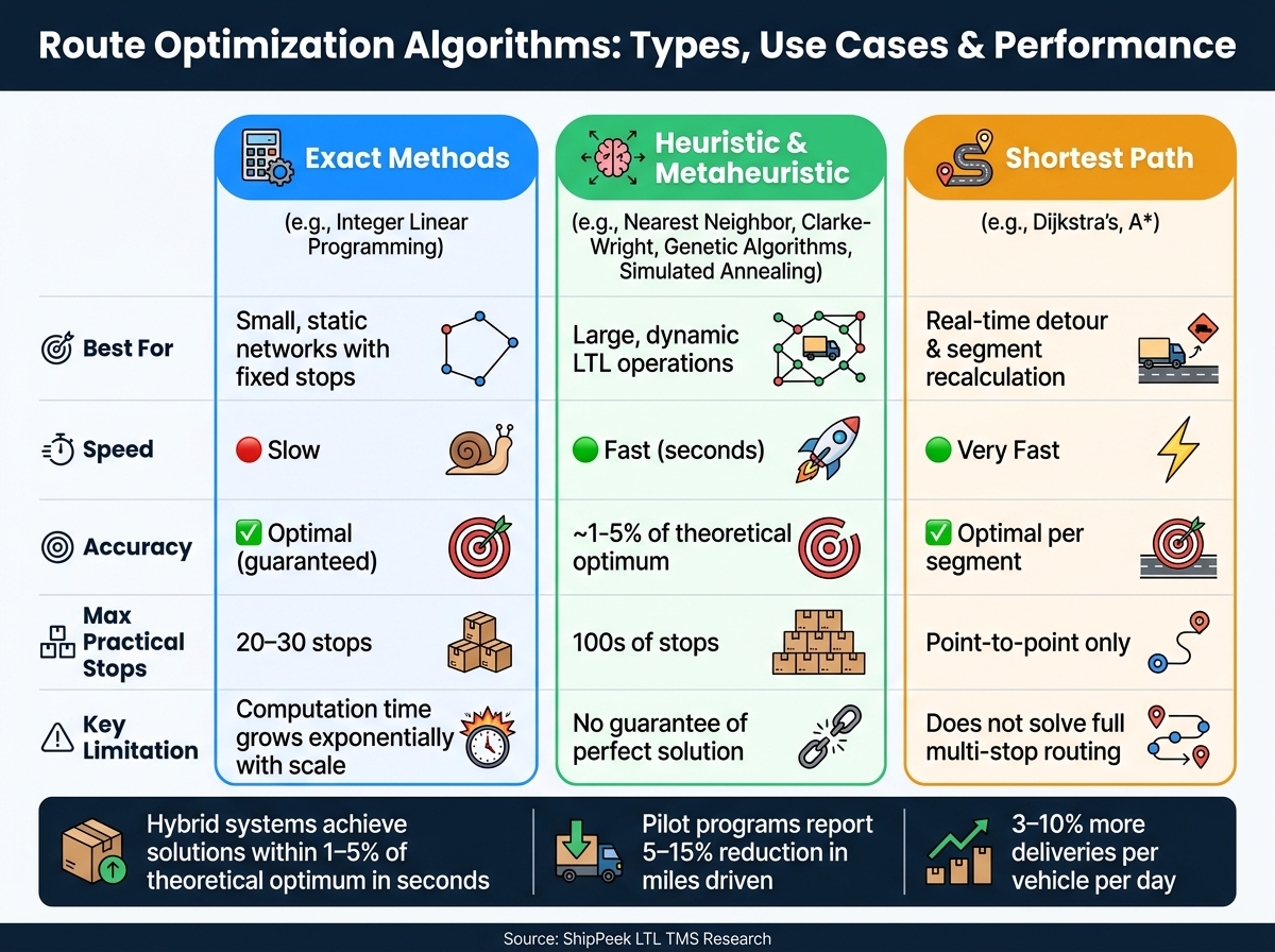
Exact Optimization Methods

Exact methods, like Integer Linear Programming (ILP), are rooted in mathematical modeling and are designed to find optimal solutions for routing problems. These methods work well for small and static networks, where the number of stops is limited. However, because Vehicle Routing Problems (VRP) are NP-hard, the computation time increases dramatically as the number of stops grows. For networks with more than 20–30 stops, solving for a guaranteed optimal route becomes almost impossible due to the computational demands [1].

As a result, exact methods are typically reserved for smaller, fixed routing tasks, such as planning daily routes for a handful of stops. They are less practical for larger, dynamic Less-Than-Truckload (LTL) operations, where faster, approximate methods are often preferred.

Heuristic and Metaheuristic Techniques

When exact methods fall short due to their computational intensity, heuristic approaches step in to provide quicker, near-optimal solutions. These methods prioritize speed over precision, making them a practical choice for larger routing challenges.

The Nearest Neighbor algorithm is one such heuristic. It builds routes by always selecting the closest unvisited stop, ensuring rapid results. However, this simplicity often leads to backtracking and inefficiencies, with routes that can be about 15% longer than the theoretical optimum for a 20-stop sequence [1].

A more refined alternative is the Clarke-Wright Savings algorithm. This method begins by treating each stop as an individual route and then merges them based on distance savings. It’s particularly effective for hub-and-spoke LTL networks, where consolidating stops into shared routes is essential for efficiency [1].

For even more complex routing challenges, metaheuristics come into play. These advanced techniques refine initial solutions and help avoid local optima. For example:

• Genetic Algorithms simulate natural selection by “breeding” the best routes and introducing random mutations to explore alternatives over thousands of iterations [1].
• Simulated Annealing uses a “temperature” variable to accept less optimal solutions early on, allowing it to explore the solution space more thoroughly before settling on a final route [1].

Modern LTL software often combines these approaches in a hybrid system. A heuristic, like Clarke-Wright, generates an initial route, while metaheuristics, such as Genetic Algorithms or Simulated Annealing, refine it further. This combination allows for solutions that are typically within 1–5% of the theoretical optimum in just seconds [1][2].

Shortest Path Algorithms

Shortest path algorithms focus on optimizing individual travel segments within a route. A classic example is Dijkstra’s algorithm, which calculates the shortest distance from a single source across a road network. While effective for static networks, it can be slower for real-time applications [2].

A* (A-Star) improves on Dijkstra by incorporating heuristics, enabling faster calculations. It’s widely used for real-time, point-to-point recalculations, making it a go-to choice for dynamic routing scenarios [2].

In LTL operations, these algorithms serve as the foundation for broader routing strategies. They provide accurate travel times and distances, which are essential inputs for VRP solvers. For instance, if a driver encounters a road closure mid-route, A* can quickly calculate a detour, ensuring the overall route remains efficient without requiring a complete re-optimization [2].

How Route Optimization Works in LTL Operations

Data Preparation and Integration

To create effective routes, the first step is ensuring the data is accurate and organized. This means removing duplicate entries, standardizing address formats, and geocoding each stop. Skipping these steps often leads to flawed results - what’s commonly known as the “garbage in, garbage out” problem - resulting in routes that are impractical to follow [4].

Once the data is cleaned, it gets integrated into the optimization engine. This is done via APIs and Geographic Information Systems (GIS), which connect systems like order management platforms, warehouse tools, and carrier networks. These integrations provide essential details, such as shipment weights, volumes, time windows for deliveries, terminal locations, and driver shift limitations [9]. Tools like ShipPeek LTL TMS simplify this process by offering real-time access to carrier data. This creates a solid, dependable foundation for building routes.

Building and Refining Routes

After the data is ready, the algorithm begins by creating an initial route. This often involves using basic methods, like the Nearest Neighbor approach, which selects the closest unvisited stop. While this provides a starting point, further refinement is necessary. Techniques like 2-opt swaps are used to eliminate inefficient segments, reducing the total distance traveled. For more complex LTL networks, advanced methods like tabu search or genetic algorithms take optimization to the next level [2].

“Advanced routing algorithms are the backbone of modern fleet operations… converting business constraints and live inputs into optimized plans that directly affect cost and service.” - Alex Mercer, Technical Product Lead [2]

Once the routes are optimized, they are continuously updated to adapt to real-world changes.

Real-Time Route Adjustments

Even the best-planned route can face unexpected challenges - traffic jams, last-minute pickups, or customer schedule changes. Modern LTL platforms tackle these issues by leveraging live GPS data, traffic updates, and incident reports to adjust routes in real time [2].

These systems differentiate between quick, minor adjustments and full-scale re-optimizations. For instance, ArcBest’s City Route Optimization (CRO) system, implemented across 240 service centers, achieved $13 million in annual savings and reduced mileage by 3.3 million miles [10].

“We learned early that it’s not about man versus machine. It’s man with machine.” - Dennis Anderson, Chief Innovation Officer, ArcBest [10]

Many platforms also include a human-in-the-loop feature, allowing dispatchers to review and, if necessary, override the automated adjustments. This collaboration between humans and technology ensures that the efficiency gains from route optimization are maintained throughout daily operations [4].

Impact of Route Optimization on LTL Efficiency

Key Performance Metrics to Track

When it comes to optimizing Less-Than-Truckload (LTL) operations, tracking the right metrics is essential. These metrics fall into three main categories: cost, service, and productivity.

Cost Metrics: Keep an eye on figures like cost per shipment, cost per mile, and total fuel spend. Fuel alone can account for up to 60% of operating expenses [5], so even a small reduction in mileage can translate into noticeable savings.

Service Metrics: Metrics like On-Time In-Full (OTIF) rate and first-attempt delivery success are critical. Why? Because customer satisfaction is on the line. Statistics show that 69% of consumers are less likely to reorder after just one late delivery, and 32% may stop doing business with a brand after one bad experience [11].

Productivity Metrics: For daily operations, focus on miles per delivery stop, stops per hour, and vehicle capacity utilization. Pilot programs often report a 5–15% reduction in miles traveled and a 3–10% increase in deliveries per vehicle [2]. Over time, these improvements can have a compounding effect across a large network.

“Route optimization isn’t just a tool; it’s the difference between steady, predictable operations and constant firefighting.” - Divya Murugan [4]

To evaluate the return on investment (ROI), use this formula:
(ΔMiles × Cost/Mile + ΔLabor × Labor Rate + ΔFuel × Price) − Implementation Cost [2]. Regularly running this calculation ensures leadership stays informed about the value being delivered.

Using ShipPeek LTL TMS for Route Optimization

Tracking these metrics is just the start; they also guide strategic adjustments to routing. But effective route optimization hinges on having accurate, real-time data - and that’s where a solid Transportation Management System (TMS) like ShipPeek LTL TMS comes in.

ShipPeek connects your systems directly to carrier networks, offering live updates on current rates, carrier availability, and shipment tracking. Its API-driven design allows for modular integration, making it perfect for modern routing needs. By separating routing computations from data retrieval, teams can perform quick recalculations without delays. This is especially helpful in LTL scenarios, where shipment volumes, delivery windows, and carrier options can change throughout the day. With unlimited rate requests and real-time tracking, ShipPeek keeps your optimization system running on the most current data.

Keeping Algorithms Up to Date

Metrics also play a role in identifying when your algorithms need a refresh. A route optimization algorithm is only as effective as the parameters it uses. Over time, road networks evolve, driver regulations change, and seasonal shifts alter freight patterns. Ignoring these changes can lead to a gradual decline in performance, often without an obvious warning sign.

To prevent this, regularly update algorithm inputs like vehicle capacities, driver shift limits, no-go zones, and delivery time windows [2]. Weekly KPI reviews can catch early warning signs, such as increased miles per delivery stop or declining OTIF rates, before they escalate into major issues [4].

Another best practice? Keep snapshots of the input data used for each routing decision. If third-party traffic feeds or geocoding services are involved, having a record of what the algorithm “saw” at the time can simplify audits and resolve billing disputes [2].

The ultimate goal is to create a system that continuously evolves, integrating real-world feedback to stay ahead of the curve.

Conclusion

Route optimization algorithms have revolutionized LTL shipping, turning hours of manual planning into efficient, automated processes. By leveraging modern hybrid approaches - blending heuristics with metaheuristics - these systems consistently achieve solutions that are just 1%–5% shy of the theoretical optimum [1]. This level of precision translates into real-world benefits: lower fuel costs, fewer empty miles, and improved on-time delivery rates.

The takeaway is clear: the complexity of LTL routing makes automation essential. Managing multiple stops, tight schedules, weight restrictions, and fluctuating carrier availability is simply too intricate for manual methods. Automated algorithms provide consistent, scalable solutions that meet these challenges head-on.

Tools like ShipPeek LTL TMS take this a step further by integrating routing logic with live carrier rates, real-time tracking, and booking capabilities. With its API-driven design, ShipPeek ensures your system uses up-to-date data, not outdated estimates, to maintain peak efficiency.

“Algorithms are, in essence, the way that human knowledge is translated into computer code so that computers can, in turn, improve human activities.” - Jim Endres, Senior Regional Account Manager, Aptean [3]

This blend of advanced algorithms and seamless data integration encapsulates the shift in LTL routing strategies. As emphasized earlier, route optimization isn’t a one-and-done task. To maintain high performance, you need clean data, well-defined rules, and regular system reviews. Continuous refinement keeps your algorithms sharp and your operations efficient.

FAQs

What data do I need for accurate route optimization?

Accurate route planning hinges on several critical pieces of information, such as exact location details for all stops, delivery time windows, and vehicle specifications like type and capacity. Incorporating real-time data - like traffic updates and road closures - allows for on-the-fly adjustments to routes. By blending static details (like schedules and destinations) with live updates, businesses can streamline planning, minimize delays, and make better use of resources while keeping customers satisfied.

Why don’t route tools always find the perfect route?

Finding the perfect route is no simple task, largely because the Vehicle Routing Problem (VRP) is incredibly complex and falls under the category of NP-hard problems. This means that solving it for large networks demands an enormous amount of computational power and time - resources that aren't practical for everyday use. To work around this, most routing tools rely on heuristic methods. These approaches help generate efficient routes quickly, but they aren't flawless. Real-world challenges like traffic conditions, strict delivery windows, and unexpected last-minute changes often make it impossible to achieve absolute perfection.

How are routes updated when traffic or stops change?

Routes are fine-tuned using real-time data and dynamic algorithms that react to changing conditions. These systems process live inputs such as traffic jams, road closures, or unexpected delays, making adjustments on the fly. Tools like GPS tracking and telematics play a key role by recalibrating routes - whether that means reordering stops or suggesting alternate paths. The result? Deliveries stay efficient, delays are minimized, and fuel costs are kept in check, even when surprises pop up.